


Article by James Le
Clothes shopping is a taxing experience. My eyes get bombarded with too much information. Sales, coupons, colors, toddlers, flashing lights, and crowded aisles are just a few examples of all the signals forwarded to my visual cortex, whether or not I actively try to pay attention. The visual system absorbs an abundance of information. Should I go for that H&M khaki pants? Is that a Nike tank top? What color are those Adidas sneakers?
Can a computer automatically detect pictures of shirts, pants, dresses, and sneakers? It turns out that accurately classifying images of fashion items is surprisingly straight-forward to do, given quality training data to start from. In this tutorial, we’ll walk through building a machine learning model for recognizing images of fashion objects using the Fashion-MNIST dataset. We’ll walk through how to train a model, design the input and output for category classifications, and finally display the accuracy results for each model.
// Image Classification
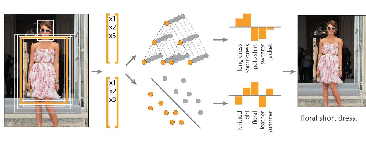
The problem of Image Classification goes like this: Given a set of images that are all labeled with a single category, we are asked to predict these categories for a novel set of test images and measure the accuracy of the predictions. There are a variety of challenges associated with this task, including viewpoint variation, scale variation, intra-class variation, image deformation, image occlusion, illumination conditions, background clutter etc.
How might we go about writing an algorithm that can classify images into distinct categories? Computer Vision researchers have come up with a data-driven approach to solve this. Instead of trying to specify what every one of the image categories of interest look like directly in code, they provide the computer with many examples of each image class and then develop learning algorithms that look at these examples and learn about the visual appearance of each class. In other words, they first accumulate a training dataset of labeled images, then feed it to the computer in order for it to get familiar with the data.
Given that fact, the complete image classification pipeline can be formalized as follows:
- Our input is a training dataset that consists of N images, each labeled with one of K different classes.
- Then, we use this training set to train a classifier to learn what every one of the classes looks like.
- In the end, we evaluate the quality of the classifier by asking it to predict labels for a new set of images that it has never seen before. We will then compare the true labels of these images to the ones predicted by the classifier.
// Convolutional Neural Networks
Convolutional Neural Networks (CNNs) is the most popular neural network model being used for image classification problem. The big idea behind CNNs is that a local understanding of an image is good enough. The practical benefit is that having fewer parameters greatly improves the time it takes to learn as well as reduces the amount of data required to train the model. Instead of a fully connected network of weights from each pixel, a CNN has just enough weights to look at a small patch of the image. It’s like reading a book by using a magnifying glass; eventually, you read the whole page, but you look at only a small patch of the page at any given time.
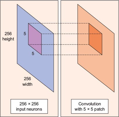
Consider a 256 x 256 image. CNN can efficiently scan it chunk by chunk — say, a 5 × 5 window. The 5 × 5 window slides along the image (usually left to right, and top to bottom), as shown below. How “quickly” it slides is called its stride length. For example, a stride length of 2 means the 5 × 5 sliding window moves by 2 pixels at a time until it spans the entire image.
A convolution is a weighted sum of the pixel values of the image, as the window slides across the whole image. Turns out, this convolution process throughout an image with a weight matrix produces another image (of the same size, depending on the convention). Convolving is the process of applying a convolution.
The sliding-window shenanigans happen in the convolution layer of the neural network. A typical CNN has multiple convolution layers. Each convolutional layer typically generates many alternate convolutions, so the weight matrix is a tensor of 5 × 5 × n, where n is the number of convolutions.
As an example, let’s say an image goes through a convolution layer on a weight matrix of 5 × 5 × 64. It generates 64 convolutions by sliding a 5 × 5 window. Therefore, this model has 5 × 5 × 64 (= 1,600) parameters, which is remarkably fewer parameters than a fully connected network, 256 × 256 (= 65,536).
The beauty of the CNN is that the number of parameters is independent of the size of the original image. You can run the same CNN on a 300 × 300 image, and the number of parameters won’t change in the convolution layer.
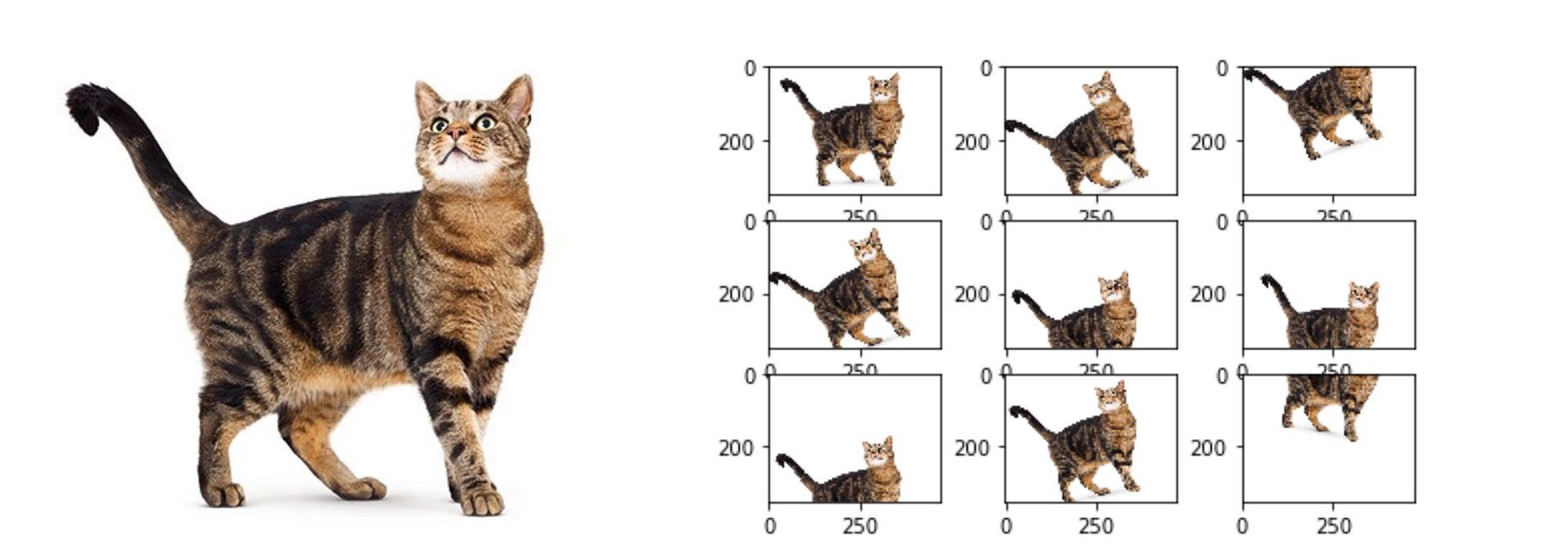
// Data Augmentation
Image classification research datasets are typically very large. Nevertheless, data augmentation is often used in order to improve generalisation properties. Typically, random cropping of rescaled images together with random horizontal flipping and random RGB colour and brightness shifts are used. Different schemes exist for rescaling and cropping the images (i.e. single scale vs. multi scale training). Multi-crop evaluation during test time is also often used, although computationally more expensive and with limited performance improvement. Note that the goal of the random rescaling and cropping is to learn the important features of each object at different scales and positions. Keras does not implement all of these data augmentation techniques out of the box, but they can easily implemented through the preprocessing function of the ImageDataGenerator modules.
// Fashion MNIST Dataset
Recently, Zalando research published a new dataset, which is very similar to the well known MNIST database of handwritten digits. The dataset is designed for machine learning classification tasks and contains in total 60 000 training and 10 000 test images (gray scale) with each 28×28 pixel. Each training and test case is associated with one of ten labels (0–9). Up till here Zalando’s dataset is basically the same as the original handwritten digits data. However, instead of having images of the digits 0–9, Zalando’s data contains (not unsurprisingly) images with 10 different fashion products. Consequently, the dataset is called Fashion-MNIST dataset, which can be downloaded from GitHub. The data is also featured on Kaggle. A few examples are shown in the following image, where each row contains one fashion item.
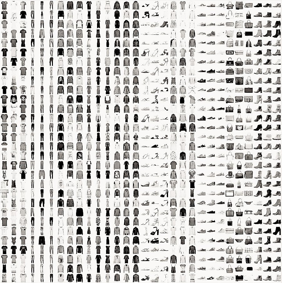
The 10 different class labels are:
- 0 T-shirt/top
- 1 Trouser
- 2 Pullover
- 3 Dress
- 4 Coat
- 5 Sandal
- 6 Shirt
- 7 Sneaker
- 8 Bag
- 9 Ankle boot
According to the authors, the Fashion-MNIST data is intended to be a direct drop-in replacement for the old MNIST handwritten digits data, since there were several issues with the handwritten digits. For example, it was possible to correctly distinguish between several digits, by simply looking at a few pixels. Even with linear classifiers it was possible to achieve high classification accuracy. The Fashion-MNIST data promises to be more diverse so that machine learning (ML) algorithms have to learn more advanced features in order to be able to separate the individual classes reliably.
// Embedding Visualization of Fashion MNIST
Embedding is a way to map discrete objects (images, words, etc.) to high dimensional vectors. The individual dimensions in these vectors typically have no inherent meaning. Instead, it’s the overall patterns of location and distance between vectors that machine learning takes advantage of. Embeddings, thus, are important for input to machine learning; since classifiers and neural networks, more generally, work on vectors of real numbers. They train best on dense vectors, where all values contribute to define an object.
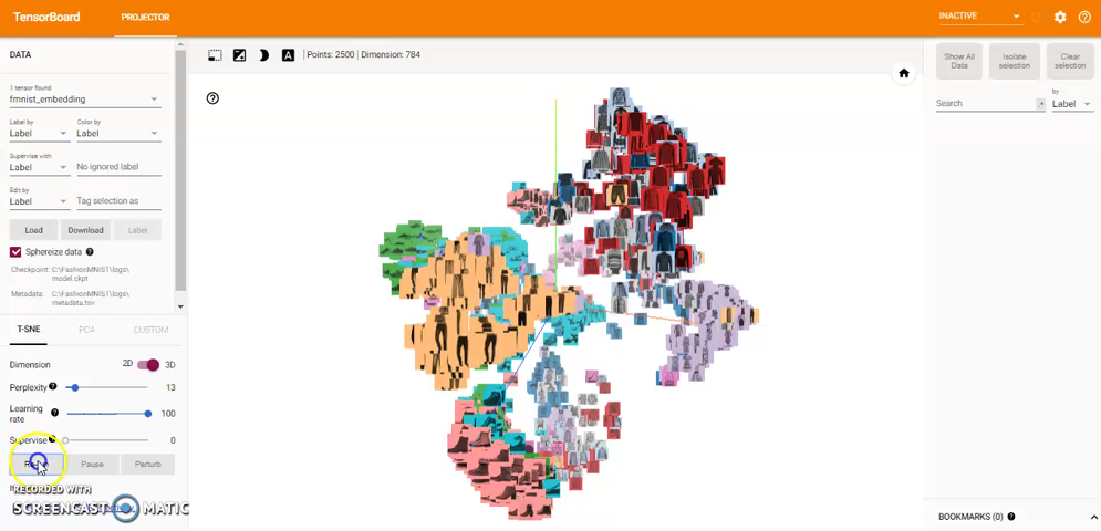
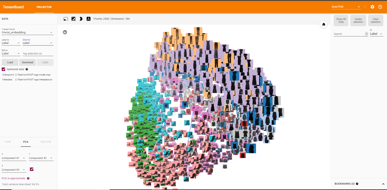
TensorBoard has a built-in visualizer, called the Embedding Projector, for interactive visualization and analysis of high-dimensional data like embeddings. The embedding projector will read the embeddings from my model checkpoint file. Although it’s most useful for embeddings, it will load any 2D tensor, including my training weights.
Here, I’ll attempt to represent the high-dimensional Fashion MNIST data using TensorBoard. After reading the data and create the test labels, I use this code to build TensorBoard’s Embedding Projector:
The Embedding Projector has three methods of reducing the dimensionality of a data set: two linear and one nonlinear. Each method can be used to create either a two- or three-dimensional view.
Principal Component Analysis: A straightforward technique for reducing dimensions is Principal Component Analysis (PCA). The Embedding Projector computes the top 10 principal components. The menu lets me project those components onto any combination of two or three. PCA is a linear projection, often effective at examining global geometry.

t-SNE: A popular non-linear dimensionality reduction technique is t-SNE. The Embedding Projector offers both two- and three-dimensional t-SNE views. Layout is performed client-side animating every step of the algorithm. Because t-SNE often preserves some local structure, it is useful for exploring local neighborhoods and finding clusters.
Custom: I can also construct specialized linear projections based on text searches for finding meaningful directions in space. To define a projection axis, enter two search strings or regular expressions. The program computes the centroids of the sets of points whose labels match these searches, and uses the difference vector between centroids as a projection axis.
You can view the full code for the visualization steps at this notebook: TensorBoard-Visualization.ipynb
// Training CNN Models on Fashion MNIST
Let’s now move to the fun part: I will create a variety of different CNN-based classification models to evaluate performances on Fashion MNIST. I will be building our model using the Keras framework. For more information on the framework, you can refer to the documentation here. Here are the list of models I will try out and compare their results:
- CNN with 1 Convolutional Layer
- CNN with 3 Convolutional Layer
- CNN with 4 Convolutional Layer
- VGG-19 Pre-Trained Model
For all the models (except for the pre-trained one), here is my approach:
- Split the original training data (60,000 images) into 80% training(48,000 images) and 20% validation (12000 images) optimize the classifier, while keeping the test data (10,000 images) to finally evaluate the accuracy of the model on the data it has never seen. This helps to see whether I’m over-fitting on the training data and whether I should lower the learning rate and train for more epochs if validation accuracy is higher than training accuracy or stop over-training if training accuracy shift higher than the validation.
- Train the model for 10 epochs with batch size of 256, compiled with categorical_crossentropy loss function and Adam optimizer.
- Then, add data augmentation, which generates new training samples by rotating, shifting and zooming on the training samples, and train the model on updated data for another 50 epochs.
Here’s the code to load and split the data:
After loading and splitting the data, I preprocess them by reshaping them into the shape the network expects and scaling them so that all values are in the [0, 1] interval. Previously, for instance, the training data were stored in an array of shape (60000, 28, 28) of type uint8 with values in the [0, 255] interval. I transform it into a float32 array of shape (60000, 28 * 28) with values between 0 and 1.
1 — 1-Conv CNN
Here’s the code for the CNN with 1 Convolutional Layer:
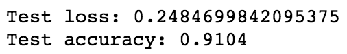
After training the model, here’s the test loss and test accuracy:
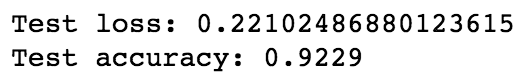
After applying data augmentation, here’s the test loss and test accuracy:
For visual purpose, I plot the training and validation accuracy and loss:
You can view the full code for this model at this notebook: CNN-1Conv.ipynb
2 — 3-Conv CNN
Here’s the code for the CNN with 3 Convolutional Layer:

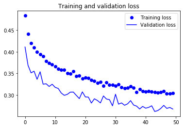
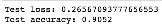
After training the model, here’s the test loss and test accuracy:

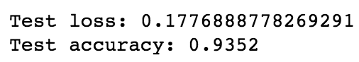
After applying data augmentation, here’s the test loss and test accuracy:
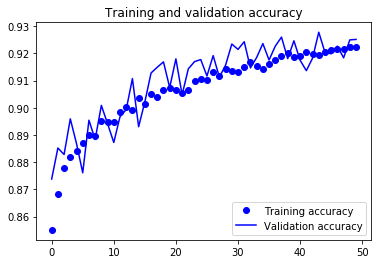
For visual purpose, I plot the training and validation accuracy and loss:
You can view the full code for this model at this notebook: CNN-3Conv.ipynb
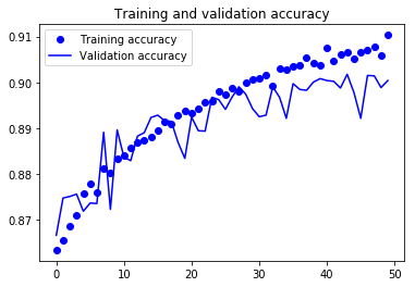
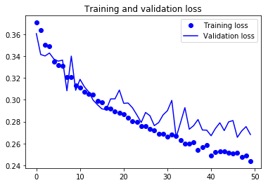
3 — 4-Conv CNN
Here’s the code for the CNN with 4 Convolutional Layer:
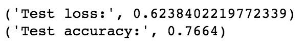
After training the model, here’s the test loss and test accuracy:
After applying data augmentation, here’s the test loss and test accuracy:
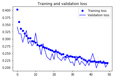
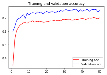
For visual purpose, I plot the training and validation accuracy and loss:
You can view the full code for this model at this notebook: CNN-4Conv.ipynb
4 — Transfer Learning
A common and highly effective approach to deep learning on small image datasets is to use a pre-trained network. A pre-trained network is a saved network that was previously trained on a large dataset, typically on a large-scale image-classification task. If this original dataset is large enough and general enough, then the spatial hierarchy of features learned by the pre-trained network can effectively act as a generic model of the visual world, and hence its features can prove useful for many different computer-vision problems, even though these new problems may involve completely different classes than those of the original task.
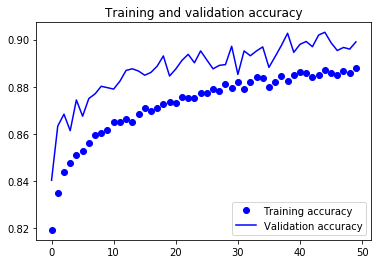
I attempted to implement the VGG19 pre-trained model, which is a widely used ConvNets architecture for ImageNet. Here’s the code you can follow:
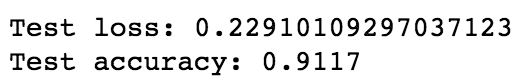
After training the model, here’s the test loss and test accuracy:
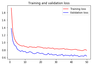
For visual purpose, I plot the training and validation accuracy and loss:
You can view the full code for this model at this notebook: VGG19-GPU.ipynb
// Last Takeaway
The fashion domain is a very popular playground for applications of machine learning and computer vision. The problems in this domain is challenging due to the high level of subjectivity and the semantic complexity of the features involved. I hope that this post has been helpful for you to learn about the 4 different approaches to build your own convolutional neural networks to classify fashion images. You can view all the source code in my GitHub repo at this link. Let me know if you have any questions or suggestions on improvement!


